QED Vacuum Birefringence Calculator

Introduction
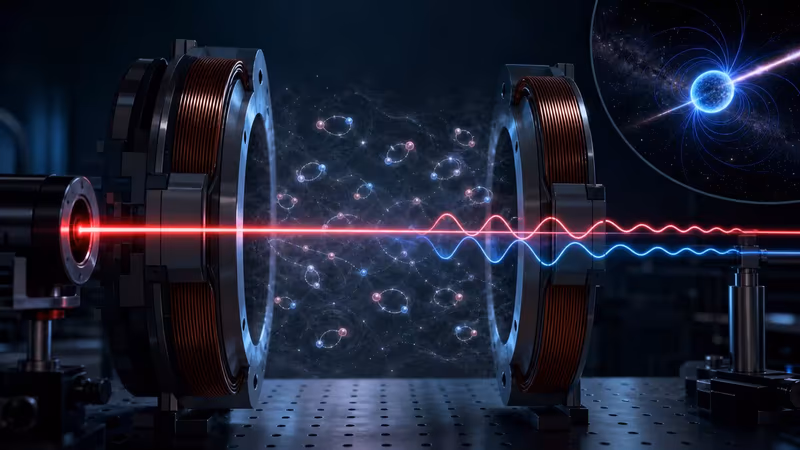
In classical electromagnetism, an empty vacuum has refractive index exactly equal to one and treats all light polarizations the same. Quantum electrodynamics changes that picture slightly. Virtual charged-particle fluctuations make the vacuum respond nonlinearly when a strong electromagnetic background field is present, so a strong magnetic field can make the vacuum behave like an extremely weak birefringent optical material.
This calculator estimates the leading-order QED vacuum birefringence for light traveling perpendicular to a uniform magnetic field. It returns the two polarization index shifts, their difference, the relative phase delay accumulated over the path length, and the small-angle ellipticity produced when the incoming linear polarization is set at 45 degrees to the field direction.
How to use this calculator
Enter the transverse magnetic field strength in tesla, the distance over which the beam remains inside that field, and the probe wavelength in nanometers. Use the physical single-pass path length unless you are intentionally modeling an effective optical-cavity path length. The wavelength should be the vacuum wavelength of the light; visible wavelengths are roughly 400 to 700 nm, while many precision optics experiments use infrared laser light such as 1064 nm.
The output is most useful for comparing orders of magnitude. Laboratory fields produce extraordinarily small signals, so a result such as 10-15 radians is not a bug. If you enter fields that approach the QED critical field, the page will flag that the weak-field approximation is no longer the right model.
Formula summary
The model uses the weak-field Euler-Heisenberg approximation: the birefringence scales with (B / Bc)2, phase delay scales with 2πL / λ, and 45-degree ellipticity is approximated as half of the relative phase delay.
Example to try
A 10 T field over 1 m with 500 nm light gives a phase delay on the order of 10-15 radians, which is why real experiments depend on long effective optical paths and careful noise control.
Limitations to check
The estimate assumes a uniform transverse magnetic field, a vacuum probe path, weak fields far below the QED critical field, and no treatment of detector noise, optical cavities, residual gas, or mirror birefringence.
Formula and method
The scale for magnetic-field nonlinearities in QED is the critical field
with Bc ≈ 4.414 × 10⁹ T. For a uniform static magnetic field, light propagating perpendicular to the field, and B much smaller than Bc, the Euler-Heisenberg effective Lagrangian gives the polarization-dependent index shifts
The birefringence is their difference,
and the phase delay over path length L at wavelength λ is
For light initially polarized at 45 degrees to the magnetic field, the small-angle ellipticity is approximately Δφ / 2. This is not the same as a Faraday rotation measurement; it is the ellipticity induced by a relative phase delay between two orthogonal polarization components.
Worked example
For a 10 T transverse magnetic field, a 1 m single-pass path length, and 500 nm light, the field ratio is about 2.27 × 10⁻⁹. The calculator gives Δn ≈ 3.97 × 10⁻²², Δφ ≈ 4.99 × 10⁻¹⁵ rad, and a 45-degree ellipticity of about 2.50 × 10⁻¹⁵ rad. Increasing the effective path length by a high-finesse cavity scales the phase delay linearly; doubling the magnetic field scales it by a factor of four.
Interpretation guide
| Quantity | Meaning | Practical note |
|---|---|---|
| n∥ - 1, n⊥ - 1 | Polarization-specific refractive-index shifts above one. | The shifts are so small that displaying the full index would round to 1 in ordinary floating-point output. |
| Δn | The birefringence between the parallel and perpendicular polarization axes. | It scales with B2, so field strength is the dominant knob. |
| Δφ | The relative phase delay accumulated over the path. | It scales with L / λ, so optical cavities and shorter wavelengths increase the signal. |
| 45-degree ellipticity | The small ellipticity estimate for an input polarization halfway between the two axes. | Real experiments must separate this signal from mirror, gas, alignment, and detector systematics. |
Assumptions and limitations
- Weak-field approximation. The formulas assume B is far below Bc. Near the critical field, this simple leading-order expression should not be used as a precision model.
- Specific geometry. The light is assumed to propagate perpendicular to a uniform, static magnetic field. Other geometries need a more general treatment.
- Vacuum only. The calculation ignores residual gas, plasma, optical coatings, mirror stress, and material birefringence. These effects can dominate in real apparatus.
- Single wavelength. The tool assumes monochromatic coherent light and does not model pulses, bandwidth, cavity mode structure, or finite coherence length.
- No experimental sensitivity model. The output is a signal estimate, not a detector design. Shot noise, modulation scheme, integration time, calibration, and systematic errors are outside the scope of this page.
FAQ
Can this calculator prove QED vacuum birefringence in a lab setup?
No. It estimates the leading-order signal size from a simplified theory model. A real experiment also needs cavity optics, modulation, detector noise, mirror birefringence, residual gas effects, calibration, and statistical analysis.
What if the magnetic field is close to the QED critical field?
The simple Euler-Heisenberg weak-field approximation used here is intended for fields far below the critical field of about 4.414 × 10⁹ T. Near or above that scale, higher-order and geometry-specific treatments are required.
Mini-game: polarization phase run
Guide the probe photon through the magnet and collect inputs that make the QED signal clearer. Dodge common impostors that would swamp the tiny vacuum birefringence signal.
Controls: move your pointer, tap a lane, or use Up and Down arrow keys.
Start the game when you are ready.